Your Brain on ChatGPT: Accumulation of Cognitive Debt when Using an AI Assistant for Essay Writing Task

# Figure 1

Figure 1. The dynamic Direct Transfer Function (dDTF) EEG analysis of Alpha Band for groups: LLM, Search Engine, Brain-only, including p-values to show significance from moderately significant (*) to highly significant (***).

# Figure 2

Figure 2. Distribution of participants' degrees.

# Figure 3

Figure 3. Distribution of participants' educational background.

# Figure 4

Figure 4. Participant during the session, while wearing Enobio headset, AttentivU headset, using BioSignal recorder software.

# Figure 5

Figure 5. Study protocol.

# Figure 6

Figure 6. Percentage of participants within each group who struggled to quote anything from their essays in Session 1.

# Figure 7

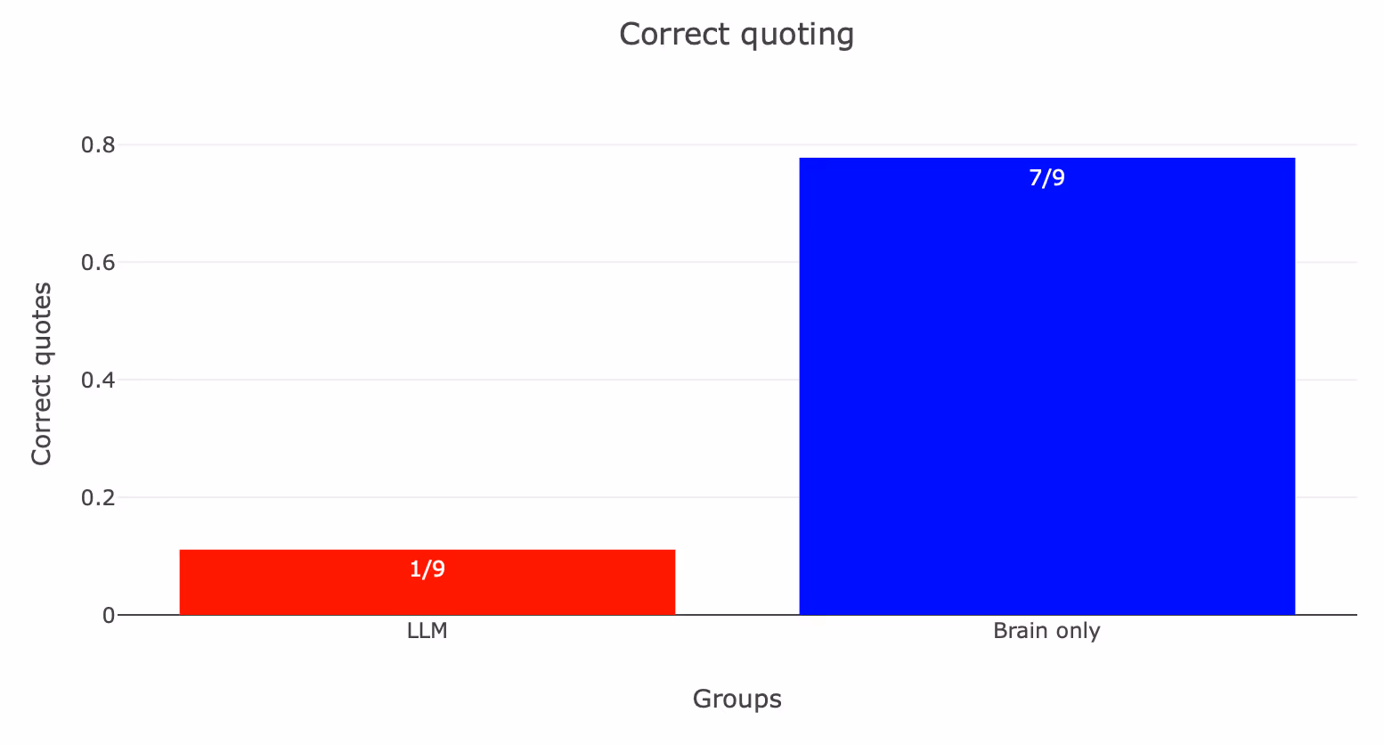
Figure 7. Percentage of participants within each group who provided a correct quote from their essays in Session 1.

# Figure 8

Figure 8. Relative reported percentage of perceived ownership of essay by the participants in comparison to the Brain-only group as a base in Session 1.

# Figure 9

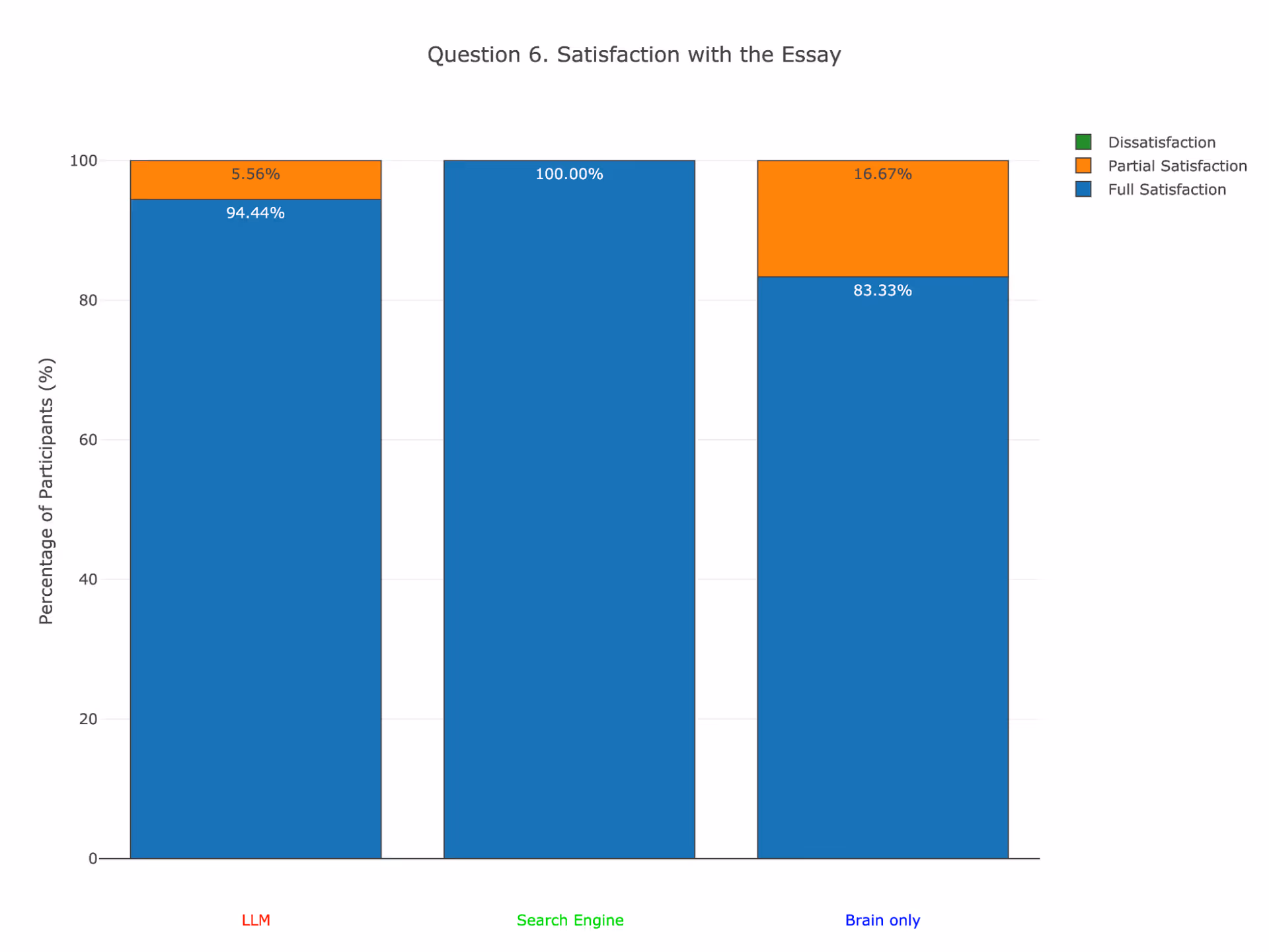
Figure 9. Reported percentage of satisfaction with the written essay by participants per group after Session 1.

# Figure 10

Figure 10. Quoting Reliability by Group in Session 4.

# Figure 11

Figure 11: Correct quoting by Group in Session 4.

# Figure 12

Figure 12. PaCMAP Distances Between the 4th Session and Previous Sessions, Averaged Per participant and Topic. This figure presents the normalized averaged PaCMAP distances between essays from the 4th session and essays from earlier sessions (1st-3rd) for the same participant and topic. Y-axis shows normalized average PaCMAP distances, representing the degree of change in essay content and structure between the 4th session and earlier ones. X-axis shows direction of session change, categorized by the writing tools used to create the essays.

# Figure 13

Figure 13. Distribution of Essays for Sessions 1,2,3 (left) and Session 4 (right) in PaCMAP XY Embedding Space Using llama4:17b-scout-16e-instruct-q4_K_M model. This figure illustrates the general distribution of essays on various topics in the PaCMAP XY embedding space, where the embeddings are generated using the LLM model. Each essay is represented by a marker, each shape represents a group: circle for LLM, square for Search Engine, and diamond for Brain-only. Each topic is assigned a distinct color to visually differentiate the distributions. Number inside each marker represents a session number.

# Figure 14

Figure 14. Distribution of Essays by Topic in PaCMAP XY Embedding Space Using llama4:17b-scout-16e-instruct-q4_K_M model. The number inside each marker represents a session number from 1 to 4.

# Figure 15

Figure 15. P values for Words per Group. This figure presents the p values for the number of words in each essay per group: LLM, Search Engine, and Brain-only. The Y-axis represents the p values, and the X-axis categorizes the groups.

# Figure 16

Figure 16. Essay length per group in number of words.

# Figure 17

Figure 17. Multi-shot system prompt for essay generation using llama4:17b-scout-16e-instruct-q4_K_M.

# Figure 18

Figure 18. Average Cosine Distance Averaged per Topic Between the Groups w.r.t. AI-Generated Essay Using the Assignment. This figure presents the average cosine distances calculated from essays across all topics comparing essays generated by participants in the Search Engine, LLM, and Brain-only groups to a standard AI-generated essay created using the same assignment using llama4:17b-scout-16e-instruct-q4_K_M. The Y-axis represents the average cosine distance, where higher values indicate greater dissimilarity from the AI-generated essay and lower values suggest greater similarity.

# Figure 19

Figure 19. Cosine Similarities in Each Group. This figure presents a heatmap of cosine similarities between the embeddings of essays generated by all participants within each group. Brain-only Group (blue), Search Engine (green), LLM (red). The heatmap visualizes the pairwise cosine similarities between the embeddings of the essays, where each cell represents the similarity between a pair of essays. Higher values (darker, closer to 1) indicate higher similarity, while lower values (lighter, closer to 0) suggest less similarity between the essays.

# Figure 20

Figure 20. KL Divergence Heatmap. This heat map illustrates the Kullback-Leibler (KL) Divergence between the n-gram distributions of essays generated by different groups within all the topics. Top-left heatmap shows averaged and aggregated KL divergence across all the topics between aggregated numbers of the n-grams in each group. The KL Divergence measures how much one distribution diverges from another, with a smoothing parameter of epsilon = 1e-10 to avoid issues with zero probabilities in the distributions. Normalised within each topic.

# Figure 21

Figure 21. NERs' Cramer's V for Topic Average. This figure shows the Cramer's V statistic for Named Entity Recognition (NER) averaged across all the topics. The Cramer's V statistic measures the strength of the association between named entities identified in the essays across different groups: LLM, Search Engine, and Brain-only. The values range from 0 (no association) to 1 (strong association), where higher values indicate a stronger consistency in the distribution of named entities.

# Figure 22

Figure 22. NER Type Frequencies for LLM. This figure shows the frequencies of different Named Entity types detected in the essays generated by the LLM group. The Y-axis represents the frequency of each NER type, while the X-axis lists the types of NERs identified in the essays.

# Figure 23

Figure 23. Named Entity Type Frequencies (NERs) for Search Engine. This figure displays the frequencies of different Named Entity types detected in the essays generated by the Search Engine group. The Y-axis represents the frequency of each NER type, while the X-axis lists the types of NERs identified in the essays.

# Figure 24

Figure 24. Named Entity Type Frequencies (NERs) for Brain-only. This figure shows the frequencies of different Named Entity types in the essays generated by the Brain-only group. The Y-axis represents the frequency of each NER type, while the X-axis lists the types of NERs detected in the essays.

# Figure 25

Figure 25. Total n-grams used across the topics per group. This figure displays a distribution of n-grams aggregated for all topics with each radius representing the frequency of the n-gram used within the topic. X axis shows most frequent ngrams. Y axis shows frequency of n-grams within the essays.

# Figure 26

Figure 26. N-grams within the FORETHOUGHT topic. This figure displays a distribution of n-grams within the FORETHOUGHT topic. X axis shows most frequent ngrams. Y axis shows frequency of n-grams within the essays.

# Figure 27

Figure 27. N-grams within the HAPPINESS topic. This figure displays a distribution of n-grams within the HAPPINESS topic. X axis shows most frequent n-grams. Y axis shows frequency of n-grams within the essays.

# Figure 28

Figure 28. System prompt for interactions classifier.

# Figure 29

Figure 29. How participants used ChatGPT before the study.

# Figure 30

Figure 30. Frequency of ChatGPT use by participants before this study.

# Figure 31

Figure 31. Distribution of ChatGPT Prompt Classifications Across Topics. This figure shows the distribution of ChatGPT prompt classifications across different topics, broken down by the frequency of each prompt type. The classifications are organized by the number of occurrences. The Y-axis shows the count of prompts in each classification, while the X-axis displays the categories arranged in descending order of frequency.

# Figure 32

Figure 32. ChatGPT prompts' classification percentage change from Sessions 1, 2, 3 to Session 4.

# Figure 33

Figure 33. Stacked Classification Distribution of ChatGPT Prompts per Topic and Intent. This figure represents a stacked bar chart illustrating the classification of ChatGPT prompts per topic and their associated intents. The X-axis is grouped by topic, and the Y-axis represents the count of prompts within each topic.

# Figure 34

Figure 34. Prompt structure of Ontology Reasoning agent based on llama4:17b-scout-16e-instruct-q4_K_M model. A simple agent was built to refine the structure and output the ontology of the input essay, including a simple feedback loop and fine system that forced LLM to produce results that can be parsed.

# Figure 35

Figure 35. Example of CHOICES Ontology. This figure illustrates an ontology for the topic of CHOICES, showing the interconnectedness of key concepts related to decision-making processes. The diagram maps out various terms such as Overchoice, Cognitive Psychology, Decisional Conflict, and others, each linked through their relationships to one another.

# Figure 36

Figure 36. Example of COURAGE Ontology. This figure illustrates an ontology for the concept of COURAGE, focusing on the relationships between various emotional and psychological elements related to vulnerability and human connection.

# Figure 37

Figure 37. Ontology of Edges per Group. This figure represents an ontology graph showing the Levenshtein distance between nodes in each group, where the edge distances are defined by a Levenshtein distance of <= 10 that we found to show enough significance across the compared edges. The Y-axis represents the "From" node, and the X-axis represents the "To" node for each edge in the ontology graph, mapping how concepts are connected within each essay group.

# Figure 38

Figure 38. Ontology Pairs Per Topic. This figure visualizes the distribution of ontology edges across topics, where the edge distances are defined by a Levenshtein distance of <= 20, which is bigger than 10 above, because we needed to have higher grouping, since we have higher number of topics compared to the number of the groups. The figure groups the edges by their respective topics, illustrating the frequency of concept pairings (or ontology pairs) within each topic. Each pairing reflects the strength of conceptual relationships between nodes within that particular topic.

# Figure 39

Figure 39. Multi-step agentic AI judge for essay scoring running on top of llama4:17b-scout-16e-instruct-q4_K_M model

# Figure 40

Figure 40. AI judge vs Human-Teacher Assessments Distribution. This scatter plot compares the average rankings given by human teachers and AI (LLM model) across different essay metrics. The X-axis represents the average scores assigned by the AI judge, while the Y-axis represents the average scores given by human teachers. Each dot on the plot corresponds to a specific essay metric, with the color of the dots differentiating between the metrics.

# Figure 41

Figure 41. AI judge vs Human Teacher Assessments. This figure compares LLM-based AI assessments with human teacher evaluations for the essays across various metrics. The Y-axis shows the average scores assigned by each assessor, with the comparison highlighting consistency and discrepancies between AI and human judgments on the same set of essays. Solid color bars show AI judge assessments, while dashed overlaid bars show human-teacher assessment per metric (each specific color). While Y axis shows aggregation per different dimensions, such as topics, sessions, group, or a combination of the above.

# Figure 42

Figure 42. Averaged Content Scores for Essays' Assessments. This figure compares the average content scores assigned by AI (LLM model) and human teachers to essays, focusing specifically on the content quality metric. The Y-axis represents the average content scores given by human teachers, while the X-axis shows the average content scores assigned by the AI judge.

# Figure 43

Figure 43. Average Structure and Organization Scores. This figure illustrates the comparison of average structure and organization scores assigned by the AI (LLM model) and human teachers across the essays. The Y-axis represents the average scores given by human teachers, while the X-axis shows the average scores given by the AI judge.

# Figure 44

Figure 44. Violin Plot of Assessments Distribution. This figure presents a violin plot illustrating the ranking distribution of essays of the Content metric, comparing AI judges and human evaluators. The plot visualizes the density of rankings across different score ranges (1-5) for both groups, providing insights into the distribution and variation in the assessments.

# Figure 45

Figure 45. Aggregated Z-Score Distribution of Assessments. This scatter plot displays the distribution of z-scores for AI judges and human evaluations, with human z-scores represented on the y-axis and AI z-scores on the x-axis. The plot offers a direct comparison of the variability in the way AI and human evaluators rate the essays across different metrics.

# Figure 46

Figure 46. Uniqueness Z-Score Heatmap of Assessments. This figure presents a heatmap illustrating the z-score distributions for teacher assessments focused on the uniqueness metric, comparing an AI model to human evaluators. The heatmap employs a color gradient to represent the density of scores across different ranges, facilitating immediate visual recognition of clustering patterns within each evaluation group. Darker colors indicate areas with higher concentrations of z-scores, while lighter colors show sparser regions. The x-axis covers the range of possible z-score values, and the y-axis distinguishes between AI judges and teacher assessments.

# Figure 47

Figure 47. Z-Score Distribution of Assessments for topic ART. This scatter plot displays the distribution of z-scores for AI judges and human evaluations, with human z-scores represented on the y-axis and AI z-scores on the x-axis. The plot offers a direct comparison of the variability in the way AI and human evaluators rate the essays across different metrics. Shapes represent different sessions, like circle is session 1, square is session 2, diamond is session 3, cross is session 4. Different fill colors represent different metrics, like yellow is uniqueness, purple is content, gray is language and style, cyan is structure and organization. Border color of each shape represents the group, like red is LLM group, Search Engine is green, and Brain-only is blue.

# Figure 48

Figure 48. Z-Score Distribution of Assessments for topic CHOICES. This scatter plot displays the distribution of z-scores for AI judges and human evaluations, with human z-scores represented on the y-axis and AI z-scores on the x-axis. The plot offers a direct comparison of the variability in the way AI and human evaluators rate the essays across different metrics. Shapes represent different sessions, like circle is session 1, square is session 2, diamond is session 3, cross is session 4. Different fill colors represent different metrics, like yellow is uniqueness, purple is content, gray is language and style, cyan is structure and organization. Border color of each shape represents the group, like red is LLM group, Search Engine is green, and Brain-only is blue.

# Figure 49

Figure 49. Z-Score Distribution of Assessments for topic COURAGE. This scatter plot displays the distribution of z-scores for AI judges and human evaluations, with human z-scores represented on the y-axis and AI z-scores on the x-axis. The plot offers a direct comparison of the variability in the way AI and human evaluators rate the essays across different metrics. Shapes represent different sessions, like circle is session 1, square is session 2, diamond is session 3, cross is session 4. Different fill colors represent different metrics, like yellow is uniqueness, purple is content, gray is language and style, cyan is structure and organization. Border color of each shape represents the group, like red is LLM group, Search Engine is green, and Brain-only is blue.

# Figure 50

Figure 50. Z-Score Distribution of Assessments for topic ENTHUSIASM. This scatter plot displays the distribution of z-scores for AI judges and human evaluations, with human z-scores represented on the y-axis and AI z-scores on the x-axis. The plot offers a direct comparison of the variability in the way AI and human evaluators rate the essays across different metrics. Shapes represent different sessions, like circle is session 1, square is session 2, diamond is session 3, cross is session 4. Different fill colors represent different metrics, like yellow is uniqueness, purple is content, gray is language and style, cyan is structure and organization. Border color of each shape represents the group, like red is LLM group, Search Engine is green, and Brain-only is blue.

# Figure 51

Figure 51. Z-Score Distribution of Assessments for topic FORETHOUGHT. This scatter plot displays the distribution of z-scores for AI judges and human evaluations, with human z-scores represented on the y-axis and AI z-scores on the x-axis. The plot offers a direct comparison of the variability in the way AI and human evaluators rate the essays across different metrics. Shapes represent different sessions, like circle is session 1, square is session 2, diamond is session 3, cross is session 4. Different fill colors represent different metrics, like yellow is uniqueness, purple is content, gray is language and style, cyan is structure and organization. Border color of each shape represents the group, like red is LLM group, Search Engine is green, and Brain-only is blue.

# Figure 52

Figure 52. Z-Score Distribution of Assessments for topic HAPPINESS. This scatter plot displays the distribution of z-scores for AI judges and human evaluations, with human z-scores represented on the y-axis and AI z-scores on the x-axis. The plot offers a direct comparison of the variability in the way AI and human evaluators rate the essays across different metrics. Shapes represent different sessions, like circle is session 1, square is session 2, diamond is session 3, cross is session 4. Different fill colors represent different metrics, like yellow is uniqueness, purple is content, gray is language and style, cyan is structure and organization. Border color of each shape represents the group, like red is LLM group, Search Engine is green, and Brain-only is blue.

# Figure 53

Figure 53. Z-Score Distribution of Assessments for topic LOYALTY. This scatter plot displays the distribution of z-scores for AI judges and human evaluations, with human z-scores represented on the y-axis and AI z-scores on the x-axis. The plot offers a direct comparison of the variability in the way AI and human evaluators rate the essays across different metrics. Shapes represent different sessions, like circle is session 1, square is session 2, diamond is session 3, cross is session 4. Different fill colors represent different metrics, like yellow is uniqueness, purple is content, gray is language and style, cyan is structure and organization. Border color of each shape represents the group, like red is LLM group, Search Engine is green, and Brain-only is blue.

# Figure 54

Figure 54. Z-Score Distribution of Assessments for topic PERFECT. This scatter plot displays the distribution of z-scores for AI judges and human evaluations, with human z-scores represented on the y-axis and AI z-scores on the x-axis. The plot offers a direct comparison of the variability in the way AI and human evaluators rate the essays across different metrics. Shapes represent different sessions, like circle is session 1, square is session 2, diamond is session 3, cross is session 4. Different fill colors represent different metrics, like yellow is uniqueness, purple is content, gray is language and style, cyan is structure and organization. Border color of each shape represents the group, like red is LLM group, Search Engine is green, and Brain-only is blue.

# Figure 55

Figure 55. Z-Score Distribution of Assessments for topic PHILANTHROPY. This scatter plot displays the distribution of z-scores for AI judges and human evaluations, with human z-scores represented on the y-axis and AI z-scores on the x-axis. The plot offers a direct comparison of the variability in the way AI and human evaluators rate the essays across different metrics. Shapes represent different sessions, like circle is session 1, square is session 2, diamond is session 3, cross is session 4. Different fill colors represent different metrics, like yellow is uniqueness, purple is content, gray is language and style, cyan is structure and organization. Border color of each shape represents the group, like red is LLM group, Search Engine is green, and Brain-only is blue.

# Figure 56

Figure 56. PaCMAP defined clusters of the interview insights between session 4 and sessions 1, 2, 3. See the insights in the appendix quoted below for each cluster on the map, top to bottom, left to right. List of descriptions is available in Appendix A.

# Figure 57

Figure 57. Dynamic Direct Transfer Function (dDTF) for Alpha band between LLM and Brain groups, only for sessions 1,2,3, excluding session 4. Rows 1 (LLM group) and 2 (Brain-only group) show the dDTF for all pairs of 32 electrodes = 1024 total. Blue is the lowest dDTF value, red is the highest dDTF value. Third row (P values) shows only significant pairs, where red ones are the most significant and blue ones are the least significant (but still below 0.05 threshold). Last two rows show only significant dDTF values filtered using the third row of p values, and normalized by the min and max ones in rows 4 and 5. Thinnest blue lines represent significant but weak dDTF values, and red thick lines represent significant and strong dDTF values.

# Figure 58

Figure 58. Dynamic Direct Transfer Function (dDTF) for Beta band between LLM and Brain groups, only for sessions 1,2,3, excluding session 4. Rows 1 (LLM group) and 2 (Brain-only group) show the dDTF for all pairs of 32 electrodes = 1024 total. Blue is the lowest dDTF value, red is the highest dDTF value. Third row (P values) shows only significant pairs, where red ones are the most significant and blue ones are the least significant (but still below 0.05 threshold). Last two rows show only significant dDTF values filtered using the third row of p values, and normalized by the min and max ones in rows 4 and 5. Thinnest blue lines represent significant but weak dDTF values, and red thick lines represent significant and strong dDTF values.

# Figure 59

Figure 59. Dynamic Direct Transfer Function (dDTF) for Delta band between LLM and Brain groups, only for sessions 1,2,3, excluding session 4. Rows 1 (LLM group) and 2 (Brain-only group) show the dDTF for all pairs of 32 electrodes = 1024 total. Blue is the lowest dDTF value, red is the highest dDTF value. Third row (P values) shows only significant pairs, where red ones are the most significant and blue ones are the least significant (but still below 0.05 threshold). Last two rows show only significant dDTF values filtered using the third row of p values, and normalized by the min and max ones in rows 4 and 5. Thinnest blue lines represent significant but weak dDTF values, and red thick lines represent significant and strong dDTF values.

# Figure 60

Figure 60. Dynamic Direct Transfer Function (dDTF) for Theta band between LLM and Brain groups, only for sessions 1,2,3, excluding session 4. Rows 1 (LLM group) and 2 (Brain-only group) show the dDTF for all pairs of 32 electrodes = 1024 total. Blue is the lowest dDTF value, red is the highest dDTF value. Third row (P values) shows only significant pairs, where red ones are the most significant and blue ones are the least significant (but still below 0.05 threshold). Last two rows show only significant dDTF values filtered using the third row of p values, and normalized by the min and max ones in rows 4 and 5. Thinnest blue lines represent significant but weak dDTF values, and red thick lines represent significant and strong dDTF values.

# Figure 61

Figure 61. Dynamic Direct Transfer Function (dDTF) for Alpha band between Search Engine and Brain-only groups, only for sessions 1,2,3, excluding session 4. Rows 1 (Search Engine group) and 2 (Brain-only group) show the dDTF for all pairs of 32 electrodes = 1024 total. Blue is the lowest dDTF value, red is the highest dDTF value. Third row (P values) shows only significant pairs, where red ones are the most significant and blue ones are the least significant (but still below 0.05 threshold). Last two rows show only significant dDTF values filtered using the third row of p values, and normalized by the min and max ones in rows 4 and 5. Thinnest blue lines represent significant but weak dDTF values, and red thick lines represent significant and strong dDTF values.

# Figure 62

Figure 62. Dynamic Direct Transfer Function (dDTF) for Beta band between Search Engine and Brain-only groups, only for sessions 1,2,3, excluding session 4. Rows 1 (Search Engine group) and 2 (Brain-only group) show the dDTF for all pairs of 32 electrodes = 1024 total. Blue is the lowest dDTF value, red is the highest dDTF value. Third row (P values) shows only significant pairs, where red ones are the most significant and blue ones are the least significant (but still below 0.05 threshold). Last two rows show only significant dDTF values filtered using the third row of p values, and normalized by the min and max ones in rows 4 and 5. Thinnest blue lines represent significant but weak dDTF values, and red thick lines represent significant and strong dDTF values.

# Figure 63

Figure 63. Dynamic Direct Transfer Function (dDTF) for Theta band between Search Engine and Brain-only groups, only for sessions 1,2,3, excluding session 4. Rows 1 (Search Engine group) and 2 (Brain-only group) show the dDTF for all pairs of 32 electrodes = 1024 total. Blue is the lowest dDTF value, red is the highest dDTF value. Third row (P values) shows only significant pairs, where red ones are the most significant and blue ones are the least significant (but still below 0.05 threshold). Last two rows show only significant dDTF values filtered using the third row of p values, and normalized by the min and max ones in rows 4 and 5. Thinnest blue lines represent significant but weak dDTF values, and red thick lines represent significant and strong dDTF values.

# Figure 64

Figure 64. Dynamic Direct Transfer Function (dDTF) for Delta band between Search Engine and Brain-only groups, only for sessions 1,2,3, excluding session 4. Rows 1 (Search Engine group) and 2 (Brain-only group) show the dDTF for all pairs of 32 electrodes = 1024 total. Blue is the lowest dDTF value, red is the highest dDTF value. Third row (P values) shows only significant pairs, where red ones are the most significant and blue ones are the least significant (but still below 0.05 threshold). Last two rows show only significant dDTF values filtered using the third row of p values, and normalized by the min and max ones in rows 4 and 5. Thinnest blue lines represent significant but weak dDTF values, and red thick lines represent significant and strong dDTF values.

# Figure 65

Figure 65. Dynamic Direct Transfer Function (dDTF) for Low Delta and High Delta bands between Search Engine and Brain-only groups, only for sessions 1,2,3, excluding session 4. Rows 1 (Search Engine group) and 2 (Brain-only group) show the dDTF for all pairs of 32 electrodes = 1024 total. Blue is the lowest dDTF value, red is the highest dDTF value. Third row (P values) shows only significant pairs, where red ones are the most significant and blue ones are the least significant (but still below 0.05 threshold). Last two rows show only significant dDTF values filtered using the third row of p values, and normalized by the min and max ones in rows 4 and 5. Thinnest blue lines represent significant but weak dDTF values, and red thick lines represent significant and strong dDTF values.

# Figure 66

Figure 66. Dynamic Direct Transfer Function (dDTF) for Low Alpha, Alpha, High Alpha bands between LLM and Search Engine groups, only for sessions 1,2,3, excluding session 4. Rows 1 (LLM group) and 2 (Search Engine group) show the dDTF for all pairs of 32 electrodes = 1024 total. Blue is the lowest dDTF value, red is the highest dDTF value. Third row (P values) shows only significant pairs, where red ones are the most significant and blue ones are the least significant (but still below 0.05 threshold). Last two rows show only significant dDTF values filtered using the third row of p values, and normalized by the min and max ones in rows 4 and 5. Thinnest blue lines represent significant but weak dDTF values, and red thick lines represent significant and strong dDTF values.

# Figure 67

Figure 67. Dynamic Direct Transfer Function (dDTF) for Alpha between LLM and Search Engine groups, only for sessions 1,2,3, excluding session 4. Rows 1 (LLM group) and 2 (Search Engine group) show the dDTF for all pairs of 32 electrodes = 1024 total. Blue is the lowest dDTF value, red is the highest dDTF value. Third row (P values) shows only significant pairs, where red ones are the most significant and blue ones are the least significant (but still below 0.05 threshold). Last two rows show only significant dDTF values filtered using the third row of p values, and normalized by the min and max ones in rows 4 and 5. Thinnest blue lines represent significant but weak dDTF values, and red thick lines represent significant and strong dDTF values.

# Figure 68

Figure 68. Dynamic Direct Transfer Function (dDTF) for Low Beta, High Beta bands between LLM and Search Engine groups, only for sessions 1,2,3, excluding session 4. Rows 1 (LLM group) and 2 (Search Engine group) show the dDTF for all pairs of 32 electrodes = 1024 total. Blue is the lowest dDTF value, red is the highest dDTF value. Third row (P values) shows only significant pairs, where red ones are the most significant and blue ones are the least significant (but still below 0.05 threshold). Last two rows show only significant dDTF values filtered using the third row of p values, and normalized by the min and max ones in rows 4 and 5. Thinnest blue lines represent significant but weak dDTF values, and red thick lines represent significant and strong dDTF values.

# Figure 69

Figure 69. Dynamic Direct Transfer Function (dDTF) for Beta band between LLM and Search Engine groups, only for sessions 1,2,3, excluding session 4. Rows 1 (LLM group) and 2 (Search Engine group) show the dDTF for all pairs of 32 electrodes = 1024 total. Blue is the lowest dDTF value, red is the highest dDTF value. Third row (P values) shows only significant pairs, where red ones are the most significant and blue ones are the least significant (but still below 0.05 threshold). Last two rows show only significant dDTF values filtered using the third row of p values, and normalized by the min and max ones in rows 4 and 5. Thinnest blue lines represent significant but weak dDTF values, and red thick lines represent significant and strong dDTF values.

# Figure 70

Figure 70. Dynamic Direct Transfer Function (dDTF) for Theta band between LLM and Search Engine groups, only for sessions 1,2,3, excluding session 4. Rows 1 (LLM group) and 2 (Search Engine group) show the dDTF for all pairs of 32 electrodes = 1024 total. Blue is the lowest dDTF value, red is the highest dDTF value. Third row (P values) shows only significant pairs, where red ones are the most significant and blue ones are the least significant (but still below 0.05 threshold). Last two rows show only significant dDTF values filtered using the third row of p values, and normalized by the min and max ones in rows 4 and 5. Thinnest blue lines represent significant but weak dDTF values, and red thick lines represent significant and strong dDTF values.

# Figure 71

Figure 71. Dynamic Direct Transfer Function (dDTF) for Low Delta, High Delta bands between LLM and Search Engine groups, only for sessions 1,2,3, excluding session 4. Rows 1 (LLM group) and 2 (Search Engine group) show the dDTF for all pairs of 32 electrodes = 1024 total. Blue is the lowest dDTF value, red is the highest dDTF value. Third row (P values) shows only significant pairs, where red ones are the most significant and blue ones are the least significant (but still below 0.05 threshold). Last two rows show only significant dDTF values filtered using the third row of p values, and normalized by the min and max ones in rows 4 and 5. Thinnest blue lines represent significant but weak dDTF values, and red thick lines represent significant and strong dDTF values.

# Figure 72

Figure 72. Dynamic Direct Transfer Function (dDTF) for Delta band between LLM and Search Engine groups, only for sessions 1,2,3, excluding session 4. Rows 1 (LLM group) and 2 (Search Engine group) show the dDTF for all pairs of 32 electrodes = 1024 total. Blue is the lowest dDTF value, red is the highest dDTF value. Third row (P values) shows only significant pairs, where red ones are the most significant and blue ones are the least significant (but still below 0.05 threshold). Last two rows show only significant dDTF values filtered using the third row of p values, and normalized by the min and max ones in rows 4 and 5. Thinnest blue lines represent significant but weak dDTF values, and red thick lines represent significant and strong dDTF values.

# Figure 73

Figure 73. Dynamic Direct Transfer Function (dDTF) for Delta band for Brain-only group, and each of the sessions 1,2,3, 4. First four rows (session 1,2,3,4) show the dDTF for all pairs of 32 electrodes = 1024 total. Blue is the lowest dDTF value, red is the highest dDTF value. Fifth row (P values) shows only significant pairs, where red ones are the most significant and blue ones are the least significant (but still below 0.05 threshold). Last four rows show only significant dDTF values filtered using the third row of p values, and normalized by the min and max ones in the last four rows. Thinnest blue lines represent significant but weak dDTF values, and red thick lines represent significant and strong dDTF values.

# Figure 74

Figure 74. Dynamic Direct Transfer Function (dDTF) for Alpha band for Brain-only group, and each of the sessions 1,2,3, 4. First four rows (session 1,2,3,4) show the dDTF for all pairs of 32 electrodes = 1024 total. Blue is the lowest dDTF value, red is the highest dDTF value. Fifth row (P values) shows only significant pairs, where red ones are the most significant and blue ones are the least significant (but still below 0.05 threshold). Last four rows show only significant dDTF values filtered using the third row of p values, and normalized by the min and max ones in the last four rows. Thinnest blue lines represent significant but weak dDTF values, and red thick lines represent significant and strong dDTF values.

# Figure 75

Figure 75. Dynamic Direct Transfer Function (dDTF) for Beta band for Brain-only group, and each of the sessions 1,2,3, 4. First four rows (session 1,2,3,4) show the dDTF for all pairs of 32 electrodes = 1024 total. Blue is the lowest dDTF value, red is the highest dDTF value. Fifth row (P values) shows only significant pairs, where red ones are the most significant and blue ones are the least significant (but still below 0.05 threshold). Last four rows show only significant dDTF values filtered using the third row of p values, and normalized by the min and max ones in the last four rows. Thinnest blue lines represent significant but weak dDTF values, and red thick lines represent significant and strong dDTF values.

# Figure 76

Figure 76. Dynamic Direct Transfer Function (dDTF) for Theta band for Brain-only group, and each of the sessions 1,2,3, 4. First four rows (session 1,2,3,4) show the dDTF for all pairs of 32 electrodes = 1024 total. Blue is the lowest dDTF value, red is the highest dDTF value. Fifth row (P values) shows only significant pairs, where red ones are the most significant and blue ones are the least significant (but still below 0.05 threshold). Last four rows show only significant dDTF values filtered using the third row of p values, and normalized by the min and max ones in the last four rows. Thinnest blue lines represent significant but weak dDTF values, and red thick lines represent significant and strong dDTF values.

# Figure 77

Figure 77. Dynamic Direct Transfer Function (dDTF) for Delta (left) and Theta (right) bands for LLM group, and each of the sessions 1,2,3, 4. First four rows (session 1,2,3,4) show the dDTF for all pairs of 32 electrodes = 1024 total. Blue is the lowest dDTF value, red is the highest dDTF value. Fifth row (P values) shows only significant pairs, where red ones are the most significant and blue ones are the least significant (but still below 0.05 threshold). Last four rows show only significant dDTF values filtered using the third row of p values, and normalized by the min and max ones in the last four rows. Thinnest blue lines represent significant but weak dDTF values, and red thick lines represent significant and strong dDTF values.

# Figure 78

Figure 78. Dynamic Direct Transfer Function (dDTF) for Beta band for LLM group, and each of the sessions 1,2,3, 4. First four rows (session 1,2,3,4) show the dDTF for all pairs of 32 electrodes = 1024 total. Blue is the lowest dDTF value, red is the highest dDTF value. Fifth row (P values) shows only significant pairs, where red ones are the most significant and blue ones are the least significant (but still below 0.05 threshold). Last four rows show only significant dDTF values filtered using the third row of p values, and normalized by the min and max ones in the last four rows. Thinnest blue lines represent significant but weak dDTF values, and red thick lines represent significant and strong dDTF values.

# Figure 79

Figure 79. Frequency distribution of n-grams between different groups and sessions for topic HAPPINESS. Left column includes n-grams. Middle column shows sessions, and the last column specifies the topic. Color lines demonstrate what tools were used: LLM (red), Search Engine (green), Brain-only (blue).

# Figure 80

Figure 80. Frequency distribution of n-grams between different groups and sessions for topic ART. Left column includes n-grams. Middle column shows sessions, and the last column specifies the topic. Color lines demonstrate what tools were used: LLM (red), Search Engine (green), Brain-only (blue).

# Figure 81

Figure 81. Frequency distribution of n-grams between different groups and sessions for topic CHOICES. Left column includes n-grams. Middle column shows sessions, and the last column specifies the topic. Color lines demonstrate what tools were used: LLM (red), Search Engine (green), Brain-only (blue).

# Figure 82

Figure 82. Frequency distribution of n-grams between different groups and sessions for topic COURAGE. Left column includes n-grams. Middle column shows sessions, and the last column specifies the topic. Color lines demonstrate what tools were used: LLM (red), Search Engine (green), Brain-only (blue).

# Figure 83

Figure 83. Frequency distribution of n-grams between different groups and sessions for topic FORETHOUGHT. Left column includes n-grams. Middle column shows sessions, and the last column specifies the topic. Color lines demonstrate what tools were used: LLM (red), Search Engine (green), Brain-only (blue). Red arrow points up to LLM-to-Brain (blue) reuse of “think before” that is actively used by LLM before.

# Figure 84

Figure 84. Frequency distribution of n-grams between different groups and sessions for topic LOYALTY. Left column includes n-grams. Middle column shows sessions, and the last column specifies the topic. Color lines demonstrate what tools were used: LLM (red), Search Engine (green), Brain-only (blue).

# Figure 85

Figure 85. Frequency distribution of n-grams between different groups and sessions for topic PERFECT. Left column includes n-grams. Middle column shows sessions, and the last column specifies the topic. Color lines demonstrate what tools were used: LLM (red), Search Engine (green), Brain-only (blue).

# Figure 86

Figure 86. Frequency distribution of n-grams between different groups and sessions for topic PHILANTHROPY. Left column includes n-grams. Middle column shows sessions, and the last column specifies the topic. Color lines demonstrate what tools were used: LLM (red), Search Engine (green), Brain-only (blue).

# Figure 87

Figure 87. Dynamic Direct Transfer Function (dDTF) for Theta band for Happiness topic between all groups. Rows 1 (LLM group), 2 (Search Engine group), and 3 (Brain-only group) show the dDTF for all pairs of 32 electrodes = 1024 total. Blue is the lowest dDTF value, red is the highest dDTF value. Fourth row (P values) shows only significant pairs, where red ones are the most significant and blue ones are the least significant (but still below 0.05 threshold). Last three rows show only significant dDTF values filtered using the third row of p values, and normalized by the min and max ones in the last three rows. Thinnest blue lines represent significant but weak dDTF values, and red thick lines represent significant and strong dDTF values.

# Figure 88

Figure 88. Dynamic Direct Transfer Function (dDTF) for Delta band for Happiness topic between all groups. Rows 1 (LLM group), 2 (Search Engine group), and 3 (Brain-only group) show the dDTF for all pairs of 32 electrodes = 1024 total. Blue is the lowest dDTF value, red is the highest dDTF value. Fourth row (P values) shows only significant pairs, where red ones are the most significant and blue ones are the least significant (but still below 0.05 threshold). Last three rows show only significant dDTF values filtered using the third row of p values, and normalized by the min and max ones in the last three rows. Thinnest blue lines represent significant but weak dDTF values, and red thick lines represent significant and strong dDTF values.

# Figure 89

Figure 89. Dynamic Direct Transfer Function (dDTF) for Alpha band for Happiness topic between all groups. Rows 1 (LLM group), 2 (Search Engine group), and 3 (Brain-only group) show the dDTF for all pairs of 32 electrodes = 1024 total. Blue is the lowest dDTF value, red is the highest dDTF value. Fourth row (P values) shows only significant pairs, where red ones are the most significant and blue ones are the least significant (but still below 0.05 threshold). Last three rows show only significant dDTF values filtered using the third row of p values, and normalized by the min and max ones in the last three rows. Thinnest blue lines represent significant but weak dDTF values, and red thick lines represent significant and strong dDTF values.

# Figure 90

Figure 90. Google Ads Keywords planner shows AI suggested bidding based on the real-time demand and supply. Higher price means higher demand. “Keywords you provided” section demonstrates preselected keywords for the price and audience breakdown. June 8, 2025.

# Figure 91

Figure 91. Probability of n-grams in the published literature according to Google N-gram viewer in books published from 1800 to 2021 (the books subset used to train OpenAI ChatGPT).

# Figure 92

Figure 92. Homeless vs Giving vs Philanthropy vs Charities in Google Trends data from 2004 to 2024.

# Appendix B

B: Dynamic Direct Transfer Function (dDTF) for Alpha band for participants 36 and 43, where they wrote on the same topic in their respective sessions using no tools or LLM. First two rows show the dDTF for all pairs of 32 electrodes = 1024 total. Blue is the lowest dDTF value, red is the highest dDTF value. Third row (P values) shows only significant pairs, where red ones are the most significant and blue ones are the least significant (but still below 0.05 threshold). Last two rows show only significant dDTF values filtered using the third row of p values, and normalized by the min and max ones in the last two rows. Thinnest blue lines represent significant but weak dDTF values, and red thick lines represent significant and strong dDTF values.